A Tactile Feedback Approach to Path Recovery after High-Speed Impacts for Collision-Resilient Drones

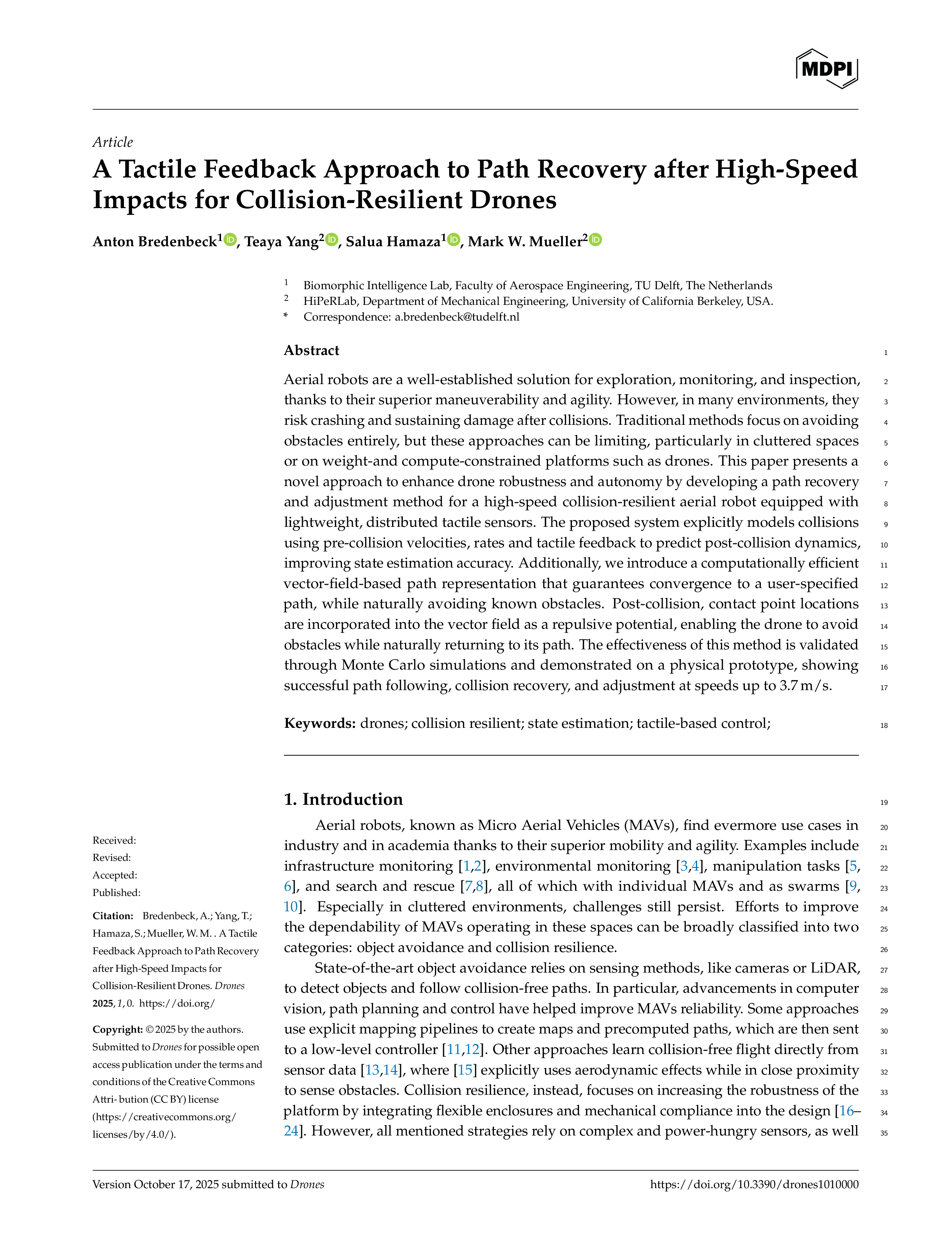

TL;DR: We equip a collision resilient quadrotor with binary contact sensors. Based on the pre-collision velocities, rates and collision points we predict the post collision velocities and rates which improves state-estimation through contact. Based on the improved state estimation and knowledge about where in the world frame the collision occured, we show improved collision recovery and path adaptation behavior.
Overview
Methods
Modelling
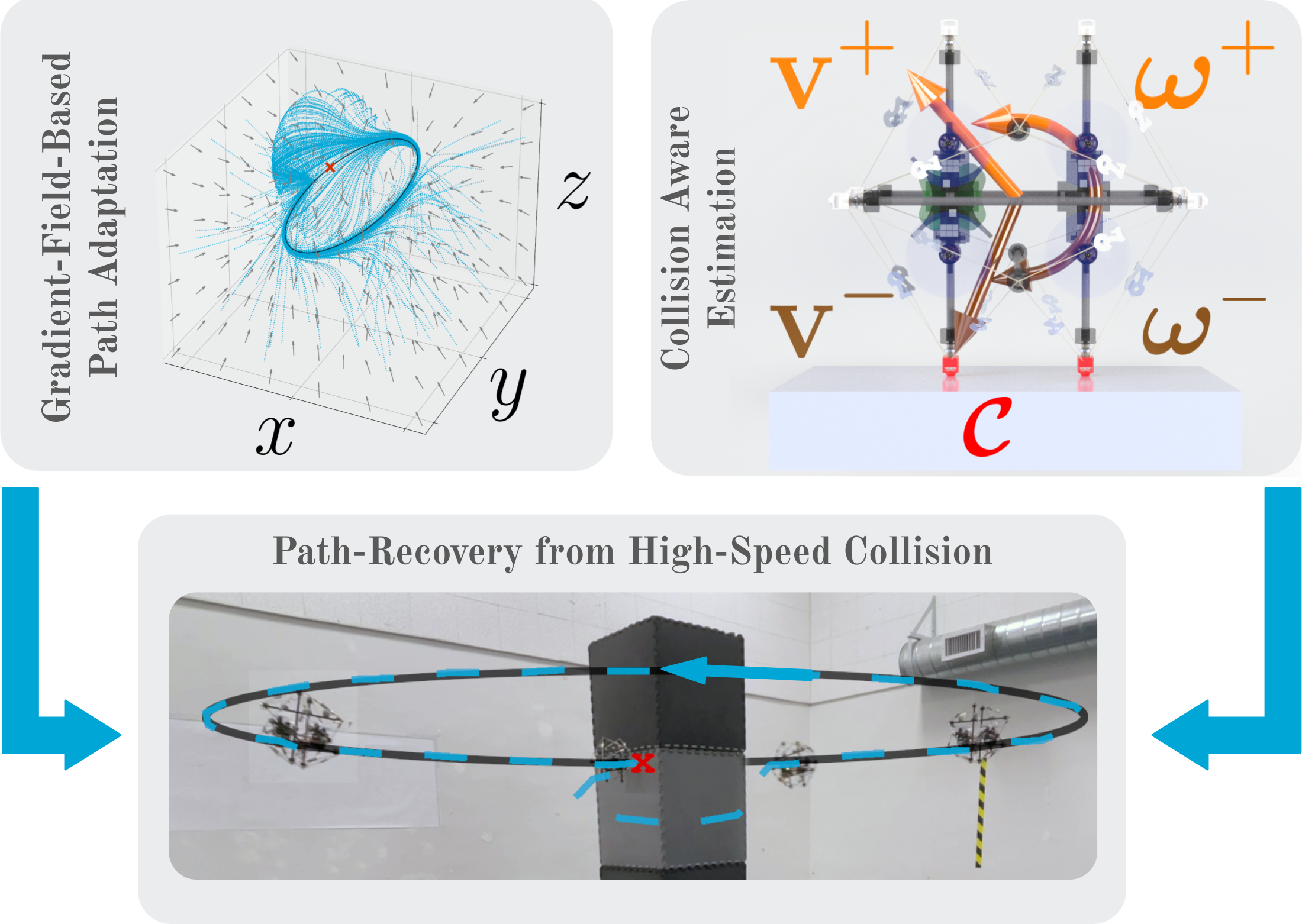
The model used is the conventional quadrotor, with its CoM encased in a protective icosahedral shell. In free flight, the system dynamics follow the standard equations of motion for a quadrotor. $$ \begin{align} \ddot{\mathbf{p}} &= m^{-1} \mathbf{f}_M + \mathbf{g}\\ \dot{\mathbf{\omega}} &= \mathbf{I}^{-1} (\mathbf{\tau}_M - \mathbf{\omega}\times\mathbf{I}\omega) \end{align} $$ The vehicle is controlled using a cascaded control approach whereby a position reference is converted into an acceleration reference, which is then translated into total thrust and attitude commands. These are subsequently tracked by a rate controller. % We assume that contact can only occur at the twelve vertices of the icosahedral shell, with the vertices treated as point contacts. Sensors detect the contact as a binary signal \(\mathbf{\mathcal{C}}\). Following an impulse-based collision modeling approach, we assume that the collision causes an instantaneous change in momentum, governed by a coefficient of restitution \(e\)and a friction coefficient \(\mu\). % For a single vertex \(i\) with the pre-collision velocity \(\mathbf{v}_{i}^- = \mathbf{v} + \mathbf{\omega}\times(\mathbf{\Omega}\mathbf{r}_i)\) the impulse \(\mathbf{j}_i\) is: $$ \begin{align} \mathbf{j}_i &= -\frac{(1+e)\langle\hat{\mathbf{n}} | \mathbf{v}_{i}^{-1}\rangle}{m^{-1} + \langle\hat{\mathbf{n}} | \mathbf{I}^{-1}(\mathbf{\Omega}\mathbf{r}_i \times \hat{\mathbf{n}})\times\mathbf{\Omega}\mathbf{r}_i\rangle}\left(\hat{\mathbf{n}} + \mu\hat{\mathbf{t}}\right) \end{align} $$ The surface normal is assumed to align with the tensegrity beam on which the active contact location lies. The friction is modeled as Coulomb, meaning it is active only if it exceeds a static threshold \(\mu_\text{static}\), which is satisfied if there is sufficient lateral velocity. The overall change in linear and angular velocity is then the normalized sum of the contribution of all \(k\) active vertices: $$ \begin{align} \Delta \mathbf{v} &= \frac{1}{k}\sum_{i=1}^k m^{-1} \mathbf{j}_i\label{eq:delta-v}\\ \Delta \mathbf{\omega} &= \frac{1}{k}\sum_{i=1}^k \mathbf{I}^{-1} \left(\mathbf{\Omega}\mathbf{r}_i\times\mathbf{j}_i\right) \label{eq:delta-omega} \end{align} $$ Normalization is required to prevent the introduction of excess energy into the system.
Contact Inclusive Estimator & Path Recovery
We employ a collision-inclusive state estimator which takes on the form of a modified Kalman Filter.
It uses a switching prediction function and assumes that, on average, the MAV follows the commanded angular velocity.
This enables the estimator's angular velocity estimate to decay toward the commanded velocity with a time constant \(\tau_\omega\).
Specifically, at each timestep \(k\), with duration \(\Delta t\), and given the commanded acceleration \(\mathbf{a}_{k, cmd}\) and angular velocity \(\mathbf{\omega}_{k,cmd}\), the prediction step proceeds as follows:
$$
\begin{align}
&\mathbf{p}_{k+1} = \mathbf{p}_k + \mathbf{v}_k \Delta t + \mathbf{a}_{k, cmd} \frac{\Delta t^2}{2}\\
&\mathbf{v}_{k+1} = \mathbf{v}_k + (1 - \kappa) \Delta t \mathbf{a}_{k, cmd} + \kappa \Delta\mathbf{v}_{\mathbf{\mathcal{C}}}\\
&\mathbf{\Omega}_{k+1} = \mathbf{\Omega}_k [\omega\Delta t]_\times\\
&\begin{aligned}
\mathbf{\omega}_{k+1} =& (1-\kappa)
\left(e^{-\frac{\Delta t}{\tau_\omega}} \omega_{k} + \left(1-e^{-\frac{\Delta t}{\tau_\omega}}\right) \mathbf{\omega}_{k, cmd}\right) \\
&+ \kappa \Delta\omega_{\mathbf{\mathcal{C}}}
\end{aligned}\\
&\kappa_{k+1} = \begin{cases}
1 & \text{if $\mathcal{C}_{i,k}$ for any $i \in [1, 12]$}\\
0 & \text{otherwise}
\end{cases},
\end{align}
$$
where \(\Delta\mathbf{v}_{\mathbf{\mathcal{C}}}\) and \(\Delta\mathbf{\omega}_{\mathbf{\mathcal{C}}}\) are the difference in linear and angular velocity due to a collision with contacts \(\mathbf{\mathcal{C}}\) as introduced before.
For any given desired (differential) path we represent then find a vector field representing the path.
Hereby the goal is to construct a vector field such that by integrating along the field one converges to the original path and moves along it while also avoiding known objects.
The vector field is initialized without any known objects and only after the reflexive collision recovery procedure in the previous section has succeeded we add the location of the triggering sensor as a new known obstacle.
The overall vector field function for a twice differential desired path \(\mathbf{h}(\tau)\) with the closest point being located at \(\mathbf{h}(\tau_\min)\) is composed of the normalized sum of three components, as illustrate below:
- One that points towards the nearest point on the path: \(\kappa_p(\mathbf{h}(\tau_{\text{min}}) - \mathbf{x})\)
- One representing the velocity at the nearest point: \(\frac{1}{\kappa_v||\mathbf{h}(\tau_{\text{min}}) - \mathbf{x}||}\mathbf{h}'(\tau_{\text{min}})\)
- One that repels from known obstacles: \(\sum_{k=1}^{m} \mathbf{g}_{\text{collision}, k}(\mathbf{x})\)
Where \(\kappa_p, \kappa_v, \mathbf{g}_{\text{collision},k}(\mathbf{x})\) are the weighting factors for position and velocity as well as the repulsive potential function for the \(k\)-th known collision. Please refer to the paper for more details on how to efficiently find the nearest point on the path.
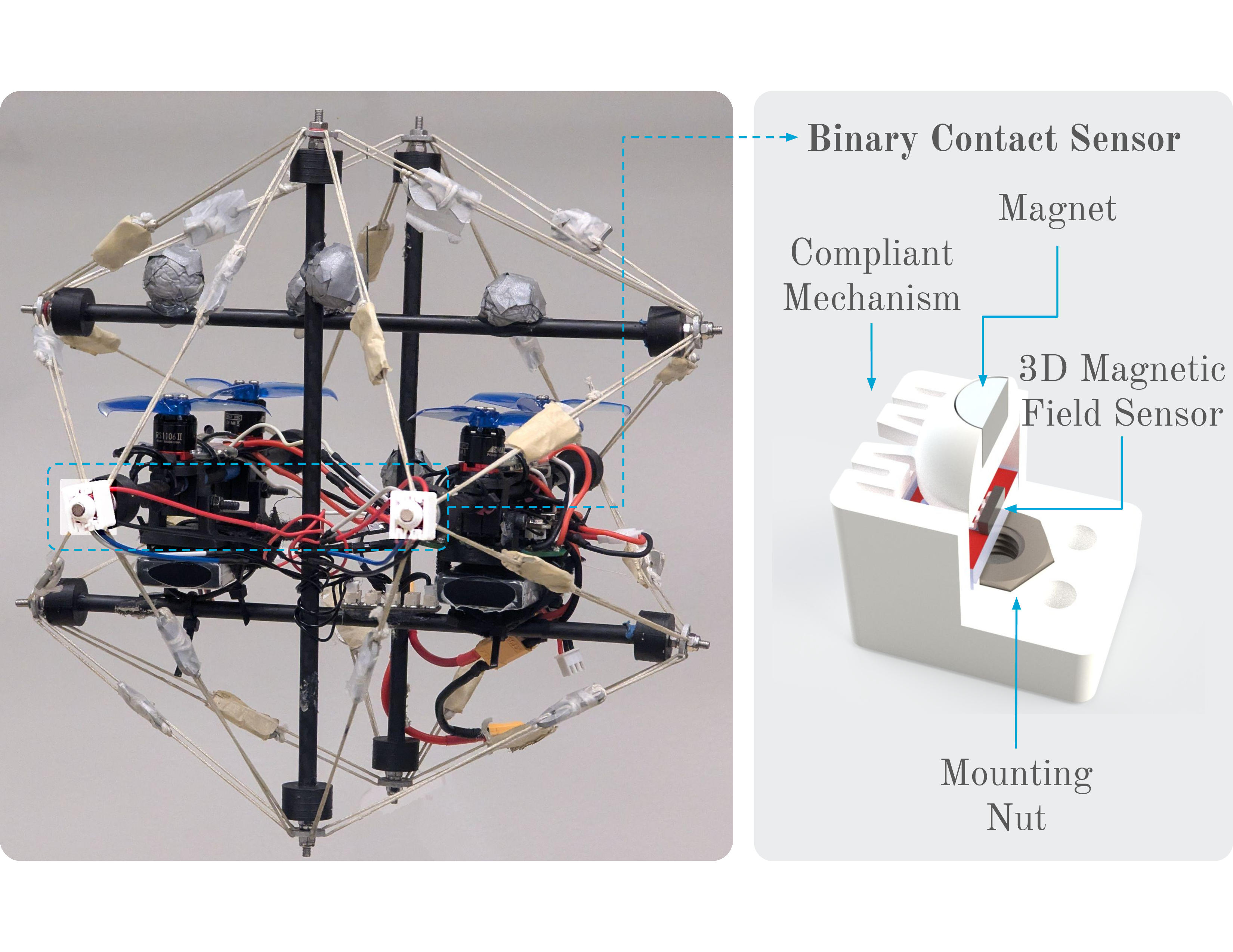
Hardware Prototype
Results
Two general scenarios are validated using Monte Carlo simulations: the first evaluates the system's ability to recover from high-speed collisions compared to non-tactile approaches, while the second assesses the reliability of the overall path-recovery procedure. The table below displays the recovery success for different velocities across three controllers: (1) a contact-agnostic cascading controller combined with a Kalman Filter, (2) the same estimator and low-level controller, but with the recovery maneuver introduced triggered when the accelerometer norm exceeds a threshold, and (3) the proposed approach. For each velocity and controller, the Monte Carlo simulation consists of 50 trials. A recovery is considered successful if the MAV does not touch the ground during the recovery maneuver. In simulation, our approach achieves a 100 % success rate for collisions up to 8 m / s, outperforming both baselines.
| Velocity (m/s) | 0.5 | 1.0 | 1.5 | 2.0 | 2.5 | 3.0 | 3.5 | 4.0 | 4.5 | 5.0 | 5.5 | 6.0 | 6.5 | 7.0 | 7.5 | 8.0 |
|---|---|---|---|---|---|---|---|---|---|---|---|---|---|---|---|---|
| Collision Agnostic | ✓ | ✗ | ✗ | ✗ | ✗ | ✗ | ✗ | ✗ | ✗ | ✗ | ✗ | ✗ | ✗ | ✗ | ✗ | ✗ |
| Accelerometer Based | ✓ | ✓ | ✓ | ✓ | ✓ | ✓ | ✗ | ✗ | ✗ | ✗ | ✗ | ✗ | ✗ | ✗ | ✗ | ✗ |
| Ours | ✓ | ✓ | ✓ | ✓ | ✓ | ✓ | ✓ | ✓ | ✓ | ✓ | ✓ | ✓ | ✓ | ✓ | ✓ | ✓ |
We evaluate the replanning capability, by commanding the MAV to take off from an initial position that is randomized for each trial by uniformly sampling from within a 50 cm cube. After takeoff, the MAV is instructed to follow an elliptical path at a speed of 1 m / s. However, this path is obstructed. The video below shows the flight paths for all \(250\) trials. The MAV successfully recovers from the collision in all trials. After recovery, it avoids the object when continuing along the path and avoids the obstacle on all subsequent passes of the elliptical trajectory. By incorporating the collision location into the vector field, the MAV naturally bypasses the obstacle and re-converges to the original path in each loop.
We further evaluate this in a simulated cluttered environment akin to a forest, as well as with more challenging obstacles, e.g. concave obstacles. In the former case the drone successfully recovers from multiple collisions and reconverges to the desired path. In the latter the drone collides multiple times with the obstacle until an escape path emerges.
We execute the same experiments on the developed prototype. Here we achieve collision recovery at speeds up to 3.7 m / s and successfully recover the elliptical path after collision as shown in the videos below.
BibTex
The website template was adapted from John Barron and Michaël Gharbi.